Are you tired of losing track of important headers while scrolling through large Excel sheets? Having knowledge for how to freeze and unfreeze panes in Excel can save you time and frustration both! This guide will tell you how to lock rows or columns in place for easy reference and fix stuck panes that won’t budge while working. Now say goodbye to scrolling chaos and hello to a smoother workflow.
How to Freeze and Unfreeze Panes in Excel (Desktop)
Tired of losing sight of important headers while scrolling through your Excel sheet? Freezing panes keep your row and column labels locked in place, making data navigation effortless. Here’s how to freeze (and unfreeze) panes in Excel quickly.
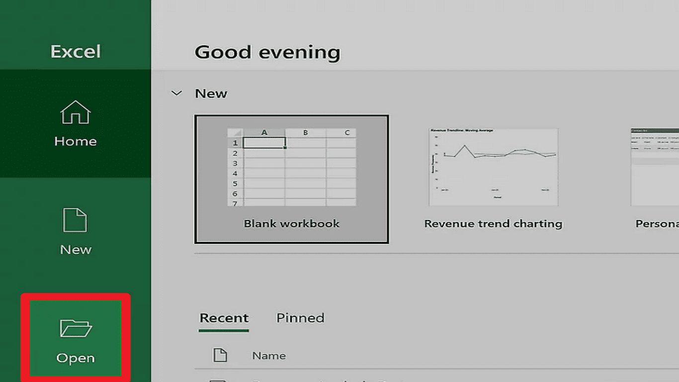
Step 1: Open Your Excel Spreadsheet
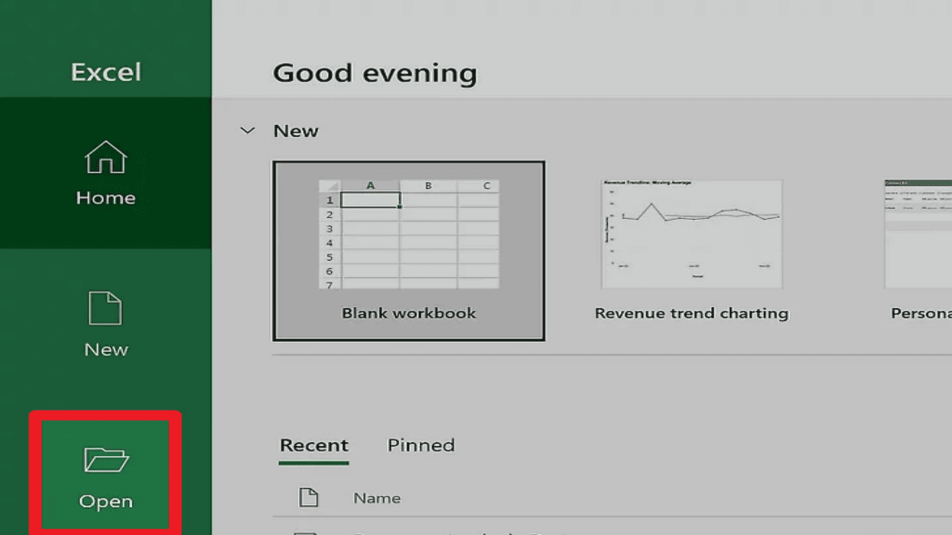
Install Microsoft Excel on your Windows or Mac computer. You can also access it online. Then, open an existing workbook or start a new one.
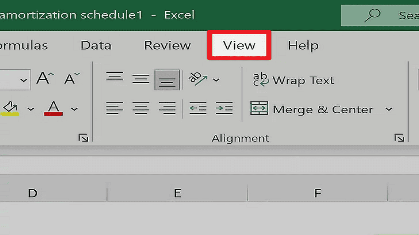
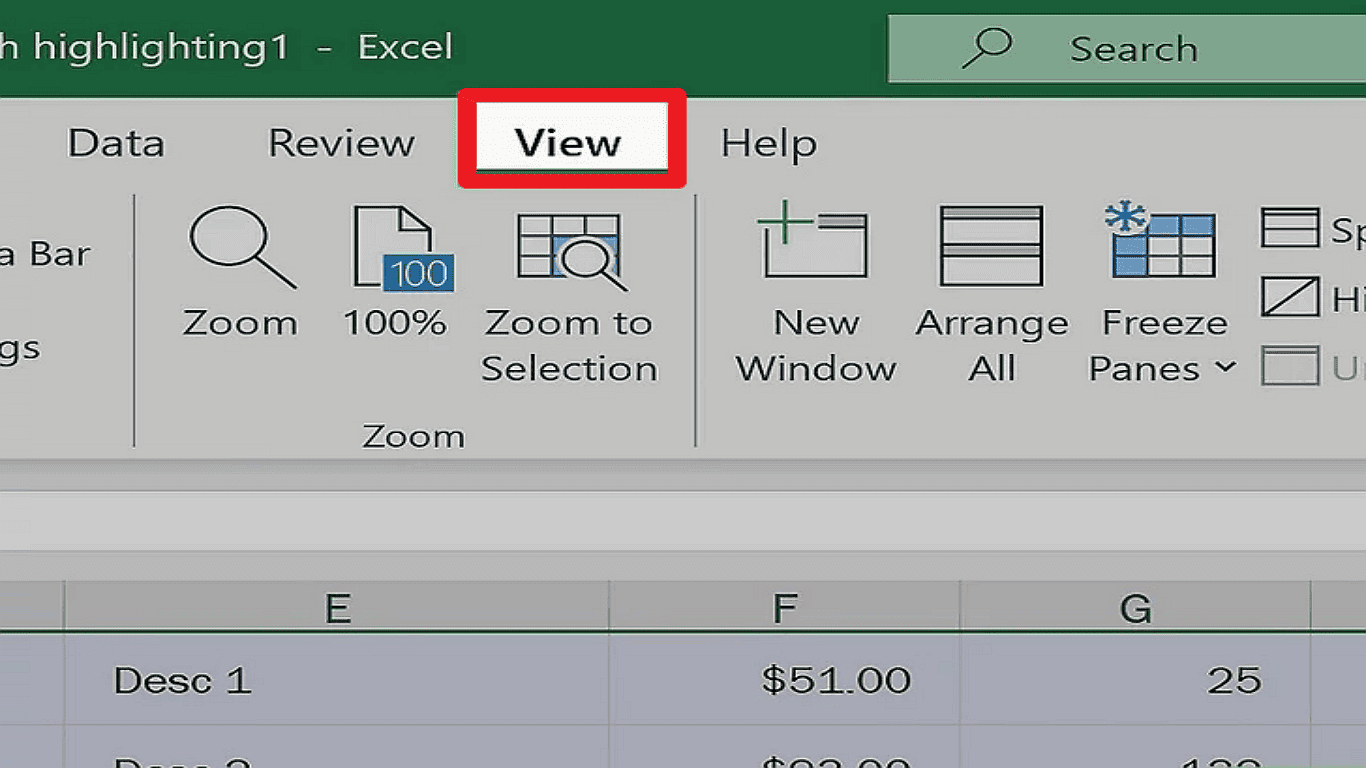
Step 2: Go to the View Tab
Now, click the View tab in the top right. You will find all the tools for managing your worksheet view.
Step 3: Click Freeze Panes
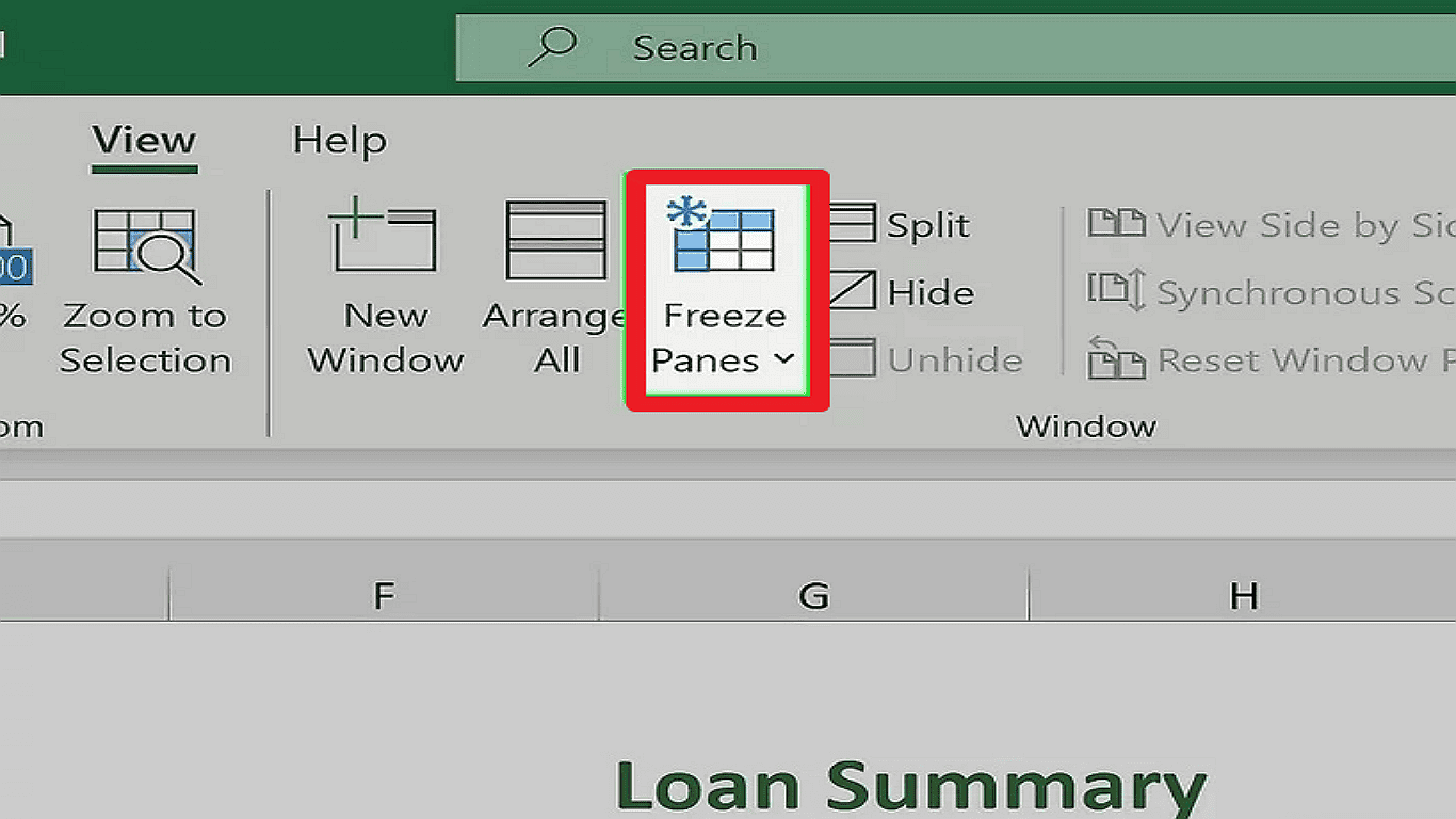
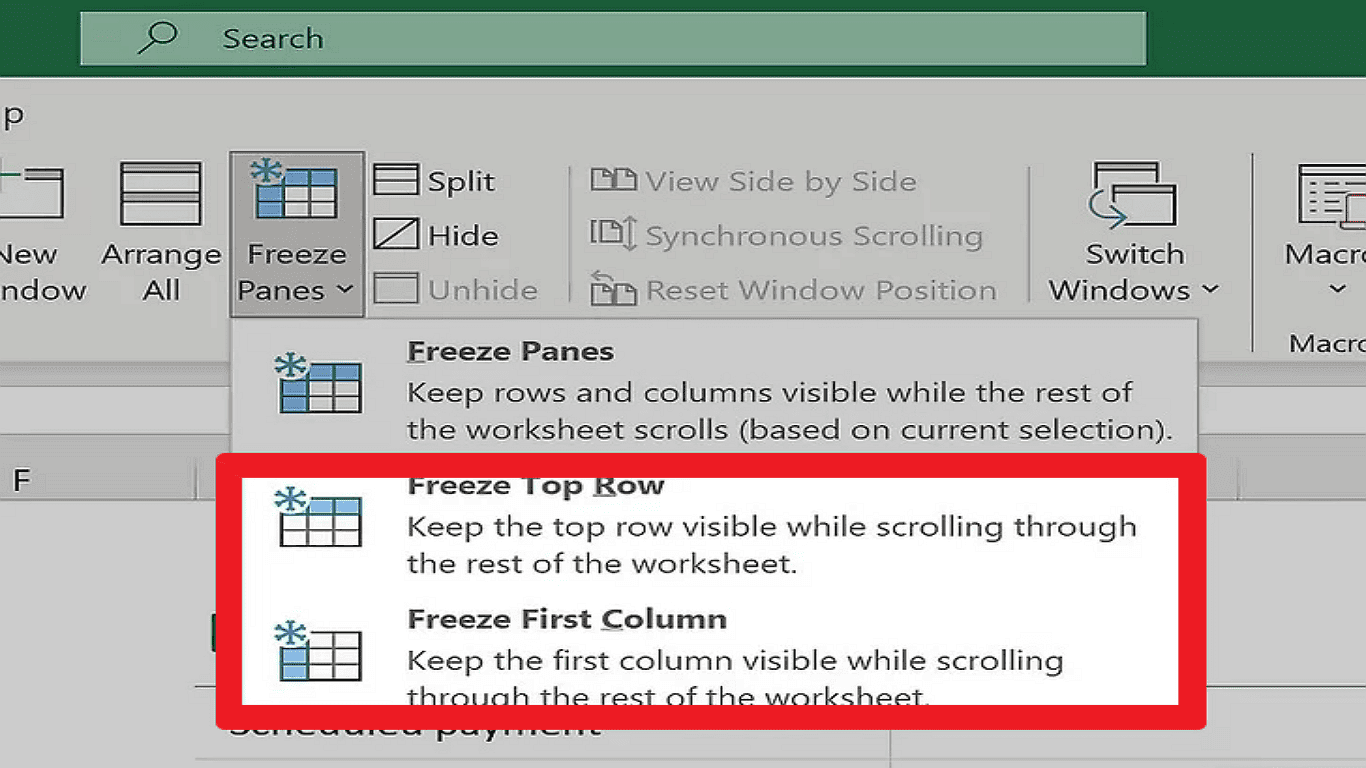
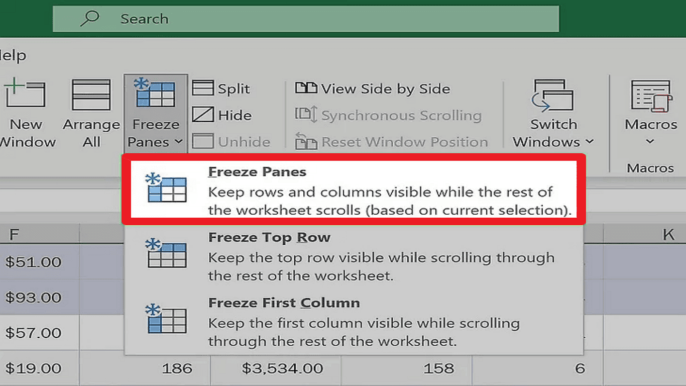
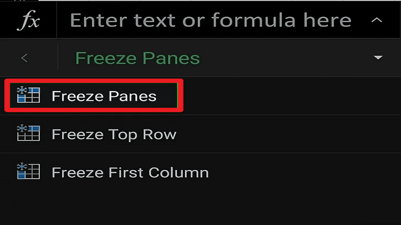
See Freeze Panes option after clicking on Window button. A dropdown menu will appear with three freezing options:
- Freeze Top Row – Locks the first row in place
- Freeze First Column – Locks the first column in place
- Freeze Panes – Let's you freeze multiple rows/columns (more advanced)
Step 4: Select Your Freezing Option
To keep your headers visible as you scroll down, choose "Freeze Top Row." If you want the first column to stay fixed while scrolling sideways, pick "Freeze First Column."
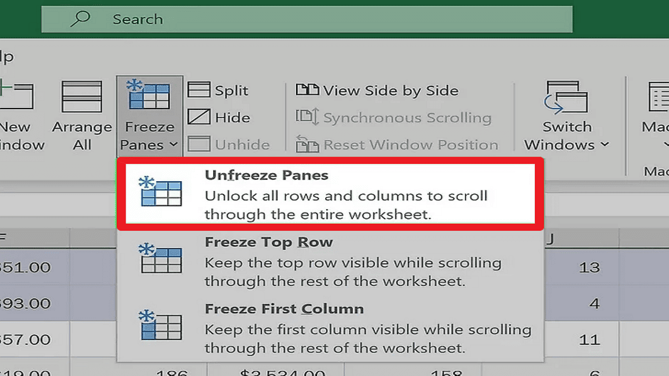
Step 5: Unfreeze Panes When Required
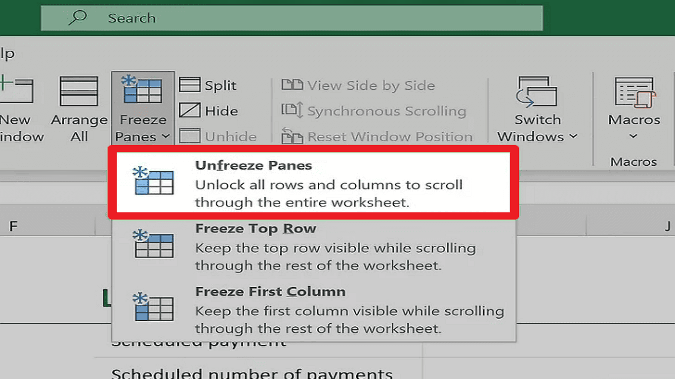
Simply go back to View > Freeze Panes > Unfreeze Panes to return to normal scrolling. This instantly releases all locked rows and columns.
Quick Tip: Excel only lets you freeze entire rows or columns—not individual cells.
Now you can navigate large datasets without losing track of your labels! For more control, check out our guide on freezing multiple panes at once.
How to Freeze and Unfreeze Multiple Rows or Columns in Excel (Desktop)
Need to keep multiple headers visible while working with large datasets? Excel's Freeze Panes feature lets you lock several rows or columns at once. Follow these simple steps to freeze (and unfreeze) multiple sections of your spreadsheet.
Step 1: Open Your Excel File
Launch Microsoft Excel and open your workbook, or create a new spreadsheet with your data.
Step 2: Select the Anchor Cell
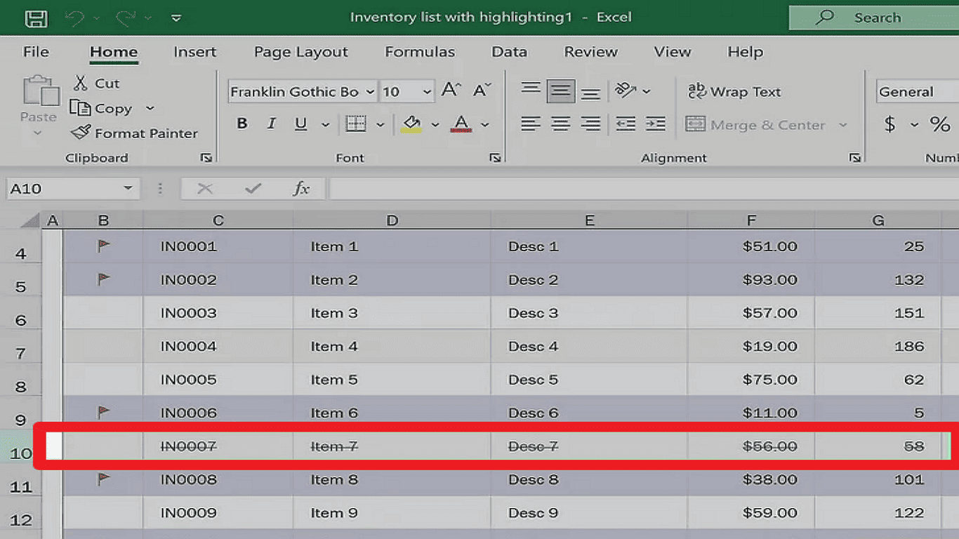
Click on the cell just below the last row and to the right of the last column you want to freeze. For example:
- To freeze rows 1-3, select row 4
- To freeze columns A-B, select column C
- To freeze both rows and columns (like A1:C3), select cell D4
You can only freeze rows/columns connected to the top or left edge of your sheet.
Step 3: Access the View Tab
Navigate to the "View" tab in Excel's top menu ribbon.
Step 4: Click Freeze Panes
In the Window group, click the "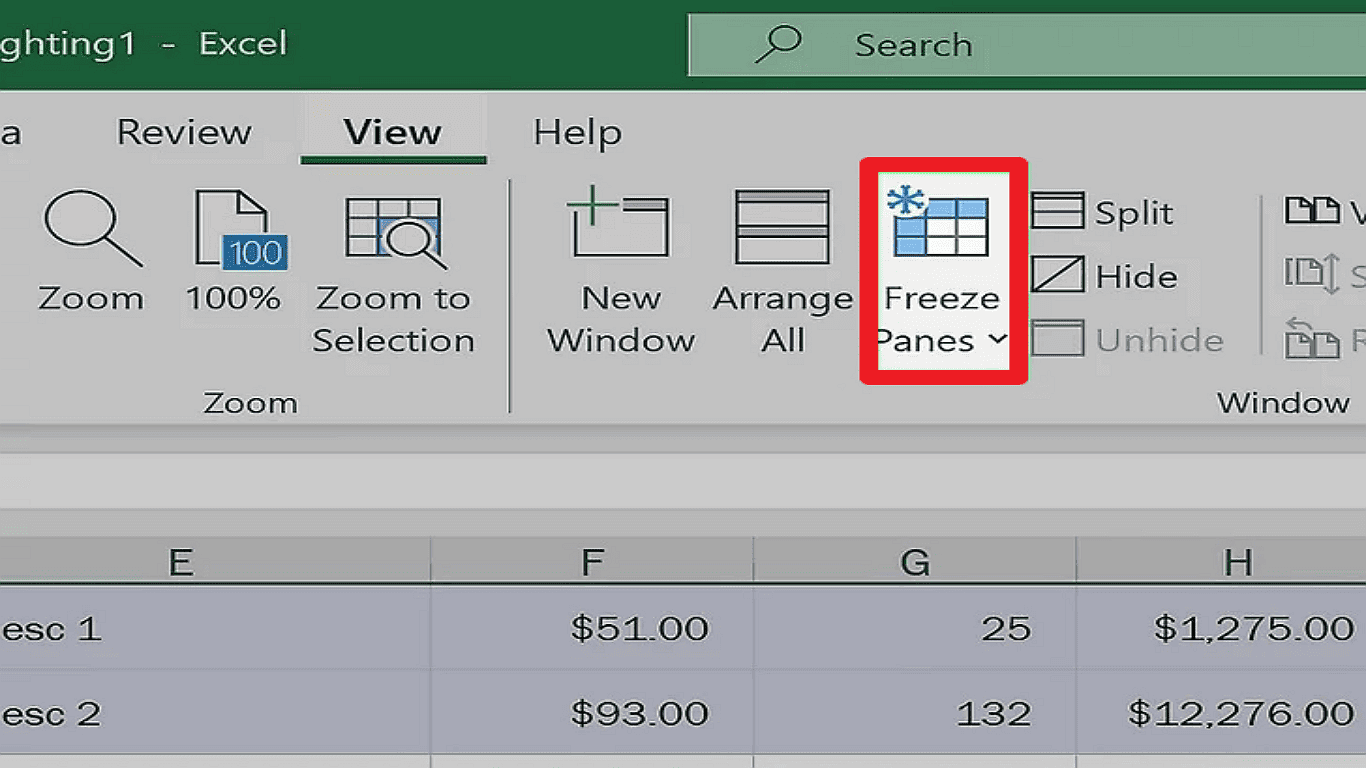 " button to reveal the dropdown options.
Step 5: Apply Freeze Panes
Select "Freeze Panes" from the menu. Excel will now lock all rows above and columns to the left of your selected cell.
Step 6: Unfreeze When Needed
Go back to View > Freeze Panes > Unfreeze Panes to remove all frozen sections.
You can use this method to keep both row and column headers visible simultaneously for large records.
Now you can scroll through extensive data while keeping your key reference points in view! For more Excel tips, check out our advanced freezing techniques guide.
How to Freeze and Unfreeze Panes in Excel Mobile (iOS/Android)
Working with spreadsheets on your phone? The Excel mobile app lets you freeze panes to keep headers visible while scrolling. Follow these simple steps to lock rows or columns in place.
Step 1: Open Your Excel File
Install the Microsoft Excel app on your iOS or Android device first. Then open an existing workbook or create a new worksheet.

Step 2: Access the View Options
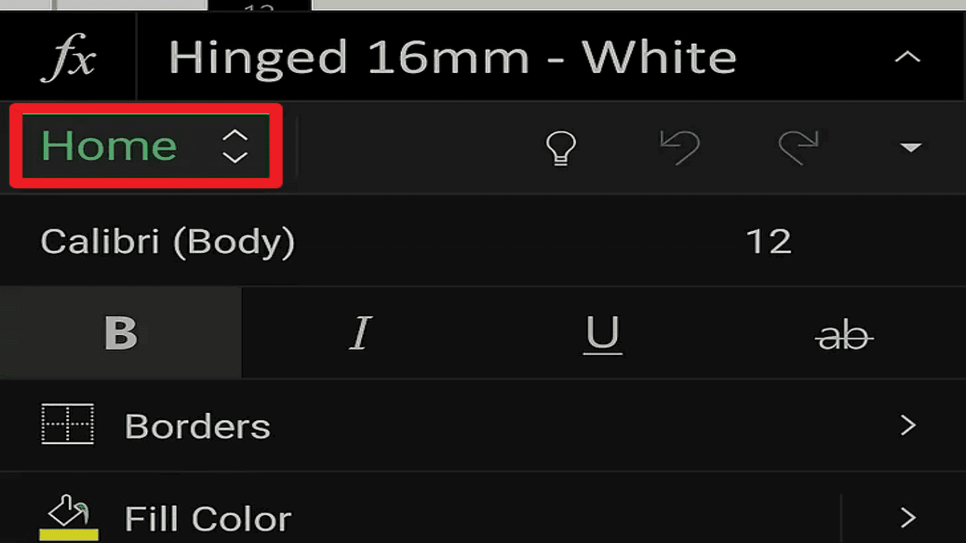
Click the Home tab at the bottom of your window. You can also tap the pencil/A icon in the top toolbar if you don't see the menu options.
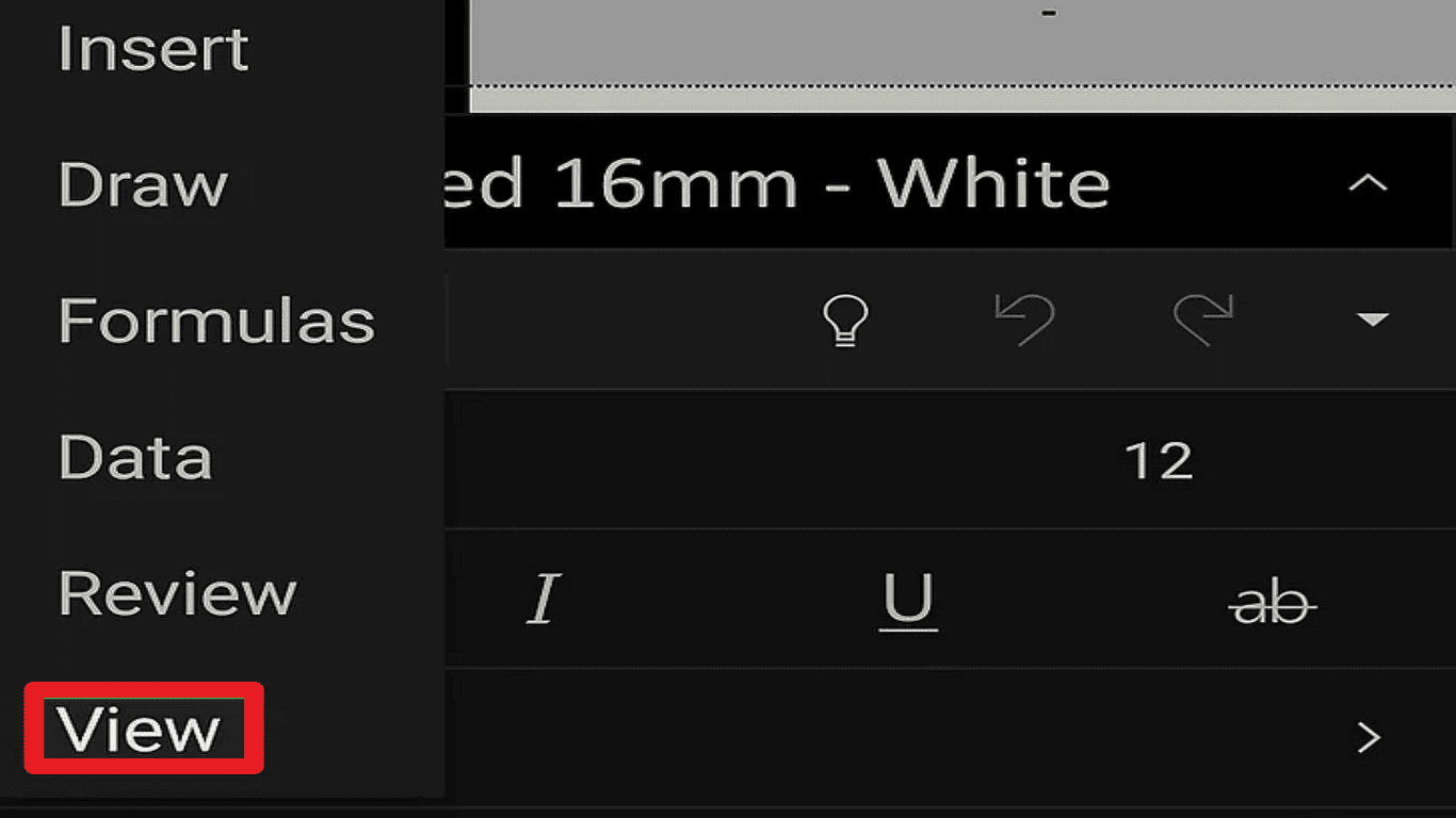
Select View from the appeared menu.
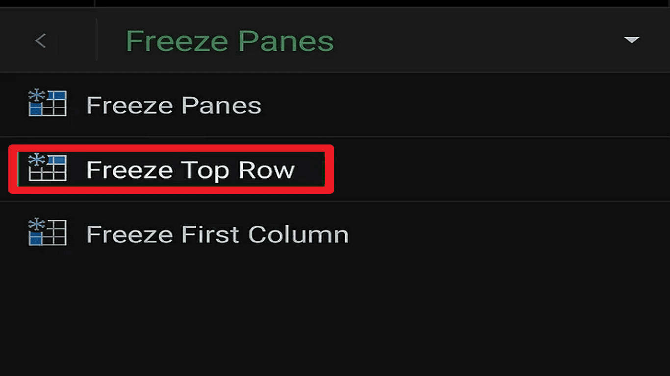
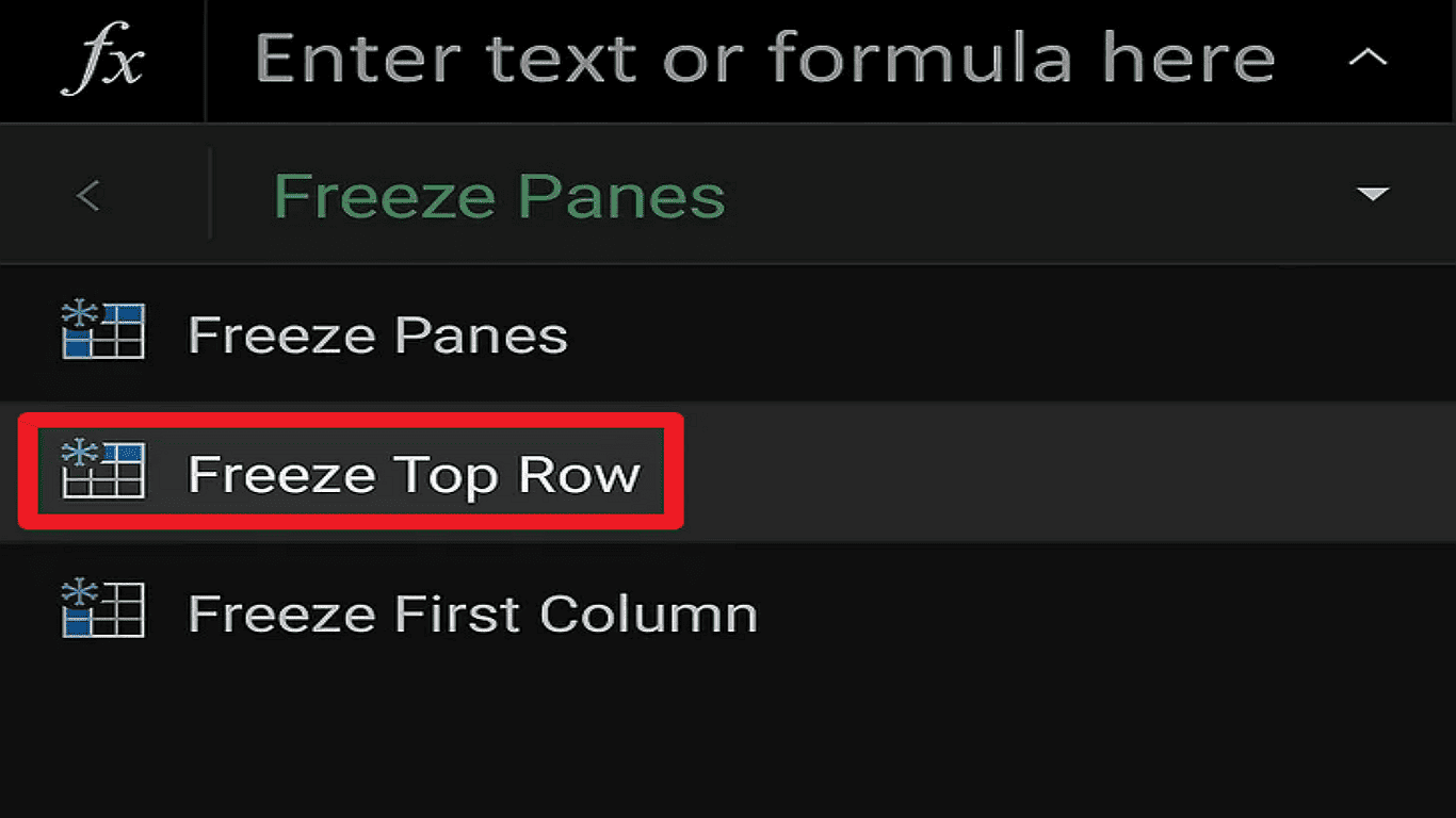
Step 3: Freeze Top Row or First Column
Pick either Freeze Top Row to lock your header row in place or Freeze First Column to keep your leftmost column visible while horizontal scrolling.
Step 4: Unfreeze Panes When Needed
Simply tap the same freeze option again to remove the checkmark and unfreeze your panes to return to normal scrolling. You can freeze multiple rows or columns for more control.
Pick the row or column immediately after the ones you want to freeze. For example:
- Tap row 4 to freeze rows 1-3
- Or column C to freeze columns A-B.
- Go to Home Tab then View
- Now click Freeze Panes to lock them.
Final Thoughts
Freezing panes are meant to enhance your workflow not to complicate it. You will discover how much time and effort they can save in your daily Excel tasks when you become more comfortable with these features. Locking specific rows and columns in place while reviewing data is just one of many powerful tools Excel offers to boost your output. For more ways to work smarter in Excel, explore our other tutorials on advanced data management and visualization techniques. Happy spreadsheeting! May your headers always stay visible and your data analysis remain frustration-free.